Artificial Intelligence (AI) has seen major breakthroughs in recent years, to a point where it can be exciting but also quite overwhelming and intimidating to start understanding, learning, and doing something with it. In this article, we’ll take a step back and look at some of the most important concepts under the AI umbrella, delve into its history, explore some of the most common types of models and model architectures, and finish it off by creating a simple model to solve a basic computer vision problem.

What is Artificial Intelligence?

In 2018, the European Commission defined AI as follows: “Artificial intelligence (AI) refers to systems that display intelligent behaviour by analysing their environment and taking actions – with some degree of autonomy – to achieve specific goals. AI-based systems can be purely software-based, acting in the virtual world (e.g. voice assistants, image analysis software, search engines, speech and face recognition systems) or AI can be embedded in hardware devices (e.g. advanced robots, autonomous cars, drones or Internet of Things applications).“. In other words, we can think of AI as the technology that enables any sort of machine, such as smartphones, cars, drones, cameras, and so on, to simulate human intelligence and problem-solving skills. 

History

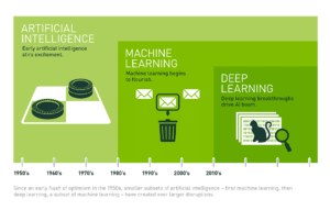
Despite some early publications and discoveries, the concept of artificial intelligence (AI) only gained traction around 1950, when pioneers like Alan Turing laid the groundwork with concepts such as the Turing Test – a test to evaluate a machine’s ability to exhibit intelligent behavior. In the years that followed, a game-playing program for checkers was developed, as well as ELIZA, a chatbot that simulated conversation and showcased the potential of AI in mimicking human interactions. Despite all of these advancements and breakthroughs, the 1970s brought a period of uncertainty and limited progress and funding known as “AI Winter”. 

In spite of this darker period, interest in AI was reignited in the 1980s with the rise of expert systems which mimicked human decision-making processes. The 1990s were marked by the win of IBM’s Deep Blue against world chess champion Garry Kasparov, while the 2000s saw the release of iRobot’s Roomba, an autonomous robot capable of vacuuming the floor while navigating and avoiding obstacles, and the growth in interest for autonomous cars. In 2012, the “ImageNet Large Scale Visual Recognition Challenge” was won by a deep learning model developed by Alex Krizhevsky, which proved to be a turning point in the years to come since existing approaches to image recognition were abandoned in favor of deep learning. 

2017 saw another turning point, when Google released the paper “Attention Is All You Need,” which introduced the concept of transformer models and revolutionized the natural language processing (NLP) field. The following year, OpenAI released GPT-1, the first version of the generative pre-trained transformer (GPT). From there onwards, generative AI began to dominate, leading to the releases of products such as ChatGPT, DALL-E, GitHub Copilot, Midjourney, Gemini, Claude, and many others. All of these advancements have significantly impacted various fields, making AI an integral part of modern technology and daily life.

Machine learning

Machine learning (ML) is a subset of AI that focuses on developing algorithms and statistical models that gradually learn to solve specific problems by recognizing patterns, connections, and correlations in data sets without the need for explicit instructions. There are five different types of machine learning techniques, each with distinct characteristics and applications: supervised learning, unsupervised learning, semi-supervised learning, self-supervised learning, and reinforcement learning.

Supervised learning

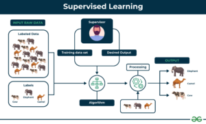
Supervised learning is the most common machine learning technique, where models are trained on a labeled dataset, meaning that the target or outcome variable is known. In an example where you have pictures of cats and dogs, the dataset provides the appropriate label (cat or dog) for each picture.

Unsupervised learning

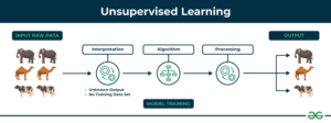
Unsupervised learning is a paradigm in which an algorithm discovers patterns and relationships using unlabeled data. The primary goal is often to discover hidden patterns, similarities, or clusters within the data, which can then be used for various purposes, such as data exploration, visualization, dimensionality reduction, and more.

Semi-supervised learning

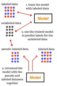
Semi-supervised learning is a technique that works between supervised and unsupervised learning since it uses both labeled and unlabeled data. It begins by developing and training a model with the labelled data available, then using the model to predict the outcome for the unlabelled data, transforming it into pseudo-labeled data, and finally retraining the model with the labelled and pseudo-labeled data combined. This technique is particularly useful and effective when obtaining labeled data is expensive, time-consuming, or resource-intensive. 

Self-supervised learning

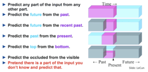
Self-supervised learning is the process where the model trains itself to learn one part of the input from another part of the input. In this process, unsupervised problems are transformed into supervised problems by the auto-generation of labels. Assume you have a dataset that includes the sentence “The capital of Portugal is Lisbon.”. This sentence alone is not very useful, but it could be used as the label or expected outcome for other sentences such as “The capital of <blank> is Lisbon.” and “The capital of Portugal is <blank>.”. For a more detailed explanation, I recommend that you watch this video, which contains an excellent explanation of this process.

Reinforcement learning

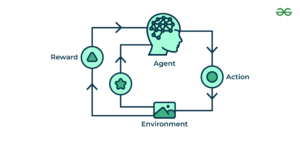
Reinforcement learning is a learning method that is used to train algorithms using a system of reward and punishment. To deploy reinforcement learning, an agent takes actions in a specific environment to reach a predetermined goal. The agent is rewarded or penalized for its actions based on an established metric, encouraging the agent to continue good practices and discard bad ones. 

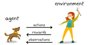
This procedure is quite similar to the process of teaching a dog to obey your commands. When your dog correctly performs a task, you reward him with a treat or his favorite toy, and when he fails to perform the action, you “punish” him by not giving him a reward and showing him what he should’ve done instead.

Deep Learning

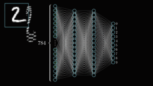
Deep learning (DL) is a subset of ML that uses multilayered neural networks, known as deep neural networks, to learn from data. These neural networks are inspired by our understanding of the biology of the human brain and try to simulate its complex decision-making capabilities.

Depending on the task that needs to be solved, there are various types of neural networks that can be used such as convolutional neural networks (CNNs), recurrent neural networks (RNNs), transformers, autoencoders, generative adversarial networks (GANs), diffusion and others. Let’s go through each one of them and understand how they work and where they can be used.

Convolutional neural networks (CNNs)

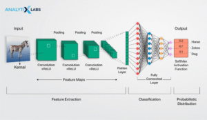
Convolutional neural networks (CNNs) specialize in processing data with a grid-like topology (e.g., an image) and are often used in tasks such as image and video recognition, image classification, and object detection. They are (mostly) composed of convolutional layers, pooling layers, and fully connected layers. Convolutional layers apply a set of filters that slide over the input image, performing a convolution operation that creates feature maps highlighting various aspects of the image, such as edges, textures, or patterns. Pooling layers, such as max pooling, reduce the spatial dimensions of the feature maps, decreasing the computational load and the number of parameters in the neural network. Fully connected layers take the features extracted by the convolutional and pooling layers and use them to make the final prediction.

Recurrent neural networks (RNNs)

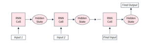
Recurrent neural networks (RNNs) are a type of neural network that are used to process sequential data. They use recurrent units to maintain a hidden state that captures information about previous elements in the sequence, allowing them to process data one step at a time. This hidden state, which essentially acts as a form of memory, is updated at each step based on the current input and the previous hidden state, enabling the network to learn patterns and dependencies in the data. RNNs can be used for tasks such as language modeling, machine translation, sentiment analysis, speech recognition, and time series prediction. However, in most of these tasks, they have been surpassed by another type of neural network called transformers.

Transformers

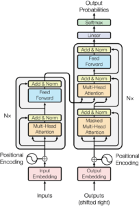
Transformers are a type of neural network that aims to solve sequence-to-sequence tasks while handling short-range and long-range dependencies in a simple way. They use a collection of mathematical approaches to detect subtle ways in which distant data elements in a series influence and depend on one another. Key components of transformers include:

• Input Embedding Layer: used to convert input data into vectors of continuous values, which are a dense representation of the input and capture the relevant properties, such as semantic and syntactic properties for text or spatial and visual features for images.
• Positional Encoding: used to provide information about the position of the input data, allowing the model to understand the relative positions within the input sequence.
• Multi-Head Attention mechanisms: allow the model to weigh the relevance of different parts of the input data by applying multiple attention heads in parallel, capturing various relationships within the data. 
• Feed-Forward Neural Networks: learn complex patterns on the data by transforming the representations produced by the self-attention mechanism.
• Normalization and Residual Connections: help to stabilize the training process by standardizing inputs to each layer and allowing gradients to flow directly from the output of a layer to its input, mitigating issues like vanishing gradients.
• Output Layer: responsible for producing the final output of the model which is achieved by converting the final vector representations into a probability distribution over the possible output tokens, generating the final output sequence.

Transformers are the state-of-the-art neural networks when it comes to NLP tasks and are the backbone of many advanced models like GPT, Gemini, Llama, and Claude. Besides NLP, they have also gained popularity and shown good results in areas such as computer vision.

Autoencoders

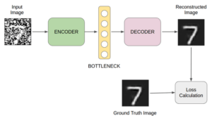
Autoencoders are a type of neural network that learns to effectively compress and encode data  and then learns to reconstruct data from a reduced encoded representation into a form that is as close as possible to the original. This type of neural network is composed by an encoder which is responsible for compressing the input data into a lower-dimensional representation, and a decoder which is responsible for reconstructing the input data from the compressed representation. The network is trained to minimize the loss function, which measures the difference between the original input and the reconstructed output. Autoencoders are quite versatile and can be used on a range of different applications, such as image denoising, anomaly detection, and data compression. 

Generative Adversarial Networks (GANs)

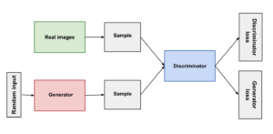
Generative Adversarial Networks (GANs) are a type of neural network capable of generating new, synthetic data that resemble real data. These networks include a generator that creates fake data from random noise that it receives as an input and a discriminator that tries to distinguish between real data that comes from the training dataset and synthetic data that is produced by the generator. These two parts work in competition, with the generator improving its creations based on probabilities that the discriminator outputs and that indicate whether the data is real or fake. The network is trained using loss functions that measure how well the generator can fool the discriminator and how well the discriminator can distinguish between real and fake data. To better understand this type of neural networks, imagine a forger trying to create a convincing fake painting, while an art expert tries to spot the forgery. The forger gets better as the expert gets harder to fool, resulting in an ever-improving fake.

GANs can be used to denoise images, to increase the resolution of images, and to generate realistic images of landscapes, people, or objects that don’t actually exist.

Diffusion

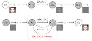
Diffusion neural networks specialize in generating high-quality data by progressively adding noise to a dataset and then learning to reverse this process. Central to their function is the forward process, which gradually adds Gaussian noise to the input data, and the reverse process, where the model learns to reverse the forward process by gradually removing the noise added, leading to the reconstruction of the original data or generation of new data. This type of neural network powers popular models such as DALL-E, Midjourney, Stable Diffusion, and Flux and is typically used for image generation.

Practical Exercise

Now that we have covered some of the history and fundamentals of AI, it is time to get our hands dirty. Our goal will be to develop a model capable of determining if the animal in a given image is a cat or a dog. As you may recall, CNNs are excellent at solving tasks related to images, so we will build a simple CNN to complete our goal.

Environment

To create this model, we will use Jupyter Notebooks in Google Collab with Python 3.10. Google Collab is a great prototyping tool since it provides a Python environment with most of the well known packages installed and it allows you to use a graphical processing unit (GPU), which speeds up the training process of your models. Although I highly recommend doing the same, you may also use Kaggle Notebooks, which is very similar to Google Collab, or do everything locally on your machine. If you choose the latter, make sure your environment has Python 3.10 and the following packages installed: numpy, Pillow, datasets and tensorflow.

Obtaining and loading data

Having large amounts of good data is very important and will be detrimental to the performance of your model, therefore you should spend a significant amount of time collecting and processing it. There are numerous ways to get data. You can look for it on sources like Hugging Face or Kaggle, use data that you already have, or collect data yourself if you don’t find anything suited for the task you want your model to perform.

In our case, we will use the datasets package from Hugging Face to load the following dataset. Sidenote: Hugging Face and Kaggle are awesome AI communities and in there you can find lots of awesome resources, so I highly recommend you bookmark them for future reference.
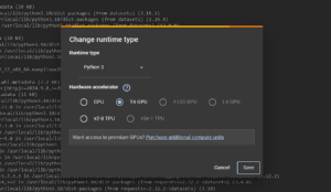
Before we start coding, we need to make sure that we are in a runtime that has access to a GPU as that will accelerate the training process of our model. To do that, go to Runtime > Change Runtime Type and select T4 GPU.

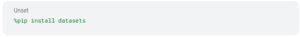
Once we have the correct runtime selected, we will install the datasets package in our notebook. We can do this be running the following in a cell:

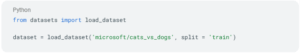
After the installation is complete, add a new cell to import the load_dataset function from the datasets package and to load the specific dataset that we want. In this case, the name of the dataset is microsoft/cats_vs_dogs and the split that we will use is train since it is the only available. Some datasets might already split the data into training data and testing data, but it is not the case with this one.

Now that we have our dataset loaded, we can inspect what is inside by simply calling it on a new cell.

And the result should the following: 

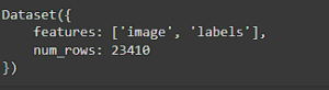
This means that the dataset has 23410 items in it, where each item contains an image and a label. You can further inspect the dataset by giving it the index and the feature that you want to see. For example, add a new cell with

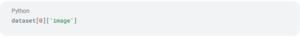
to see the image of the first item on the dataset (for index 0 it is the picture of a cat). To view the label you can do the same thing, but just replace image with labels. This will show 0 if the image on that index is a cat or 1 if the image is a dog.

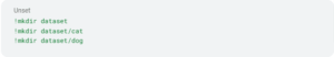
Now, let’s save the images on the disk. Firstly we will create some folders by running the following in a new cell:

And afterwards run the following in another new cell:

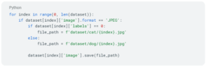
This saves all the cat images under the dataset/cat directory and all the dog images under the dataset/dog directory.

Now let’s divide the dataset into two sets: training and validation. When training a model, you should not use all the data; instead, use a larger amount for training and a smaller one for validation. This ensures that the model does not focus only on learning from a specific dataset but also performs well when faced with new and unseen data. In this scenario, we will use 75% of the data for training and 25% for validation.
To split the data, we will use a utility function called image_dataset_from_directory from TensorFlow, which is the package that we will use to create and train our model since it specializes in numerical computation, large-scale ML, DL, and other statistical and predictive analytics workloads. In order to do so, add a new cell with the following code:

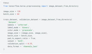
In summary, this code:

• loads the images and infers the labels from the dataset directory (labels, label_mode)
• converts the images to grayscale (color_mode)
• resizes the images to 128 of width and 128 of height (image_size)
• pads the images so that they are not deformed from the resize (pad_to_aspect_ratio)
• defines the number of samples processed in one iteration of training (batch_size) 
• splits the dataset into a training set that contains 75% of the images and a validation set that contains the remaining 25% (validation_split)
• defines the shape of each image (data_format)

Now that we have our data ready, it is time to create and train our model.

Model creation and training

TensorFlow includes a high-level API called Keras to facilitate model creation. Keras allows you to build models using either a functional or sequential approach. For this example, let’s use the sequential approach. At this point, we can already import all the layers that we will need as well as define the input layer.

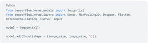
In the input layer, we define the format that it will accept, which in this case is the image width and height (both 128) as well as the number of channels. In our situation, we will choose 1 as the number of channels because we are using grayscale images; however, if you have a scenario where you use colored images, set it to 3.

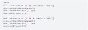
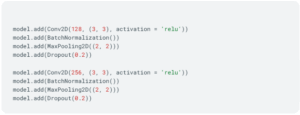
Now that we have the input layer defined, let’s add some convolutional blocks to our model. These convolutional blocks will be formed by 4 types of layers: 

• Conv2D: layer that extracts features by applying a set of learnable filters, enabling the network to detect various features such as edges, textures, and patterns
• BatchNormalization: layer used to improve the stability and performance of neural networks as it normalizes the activations of each layer
• MaxPooling2D: layer that selects the maximum value from each region of the feature map. This type of layer is a way to downsample the feature maps produced by convolutional layers, reducing the spatial dimensions and computational complexity of the network
• Dropout: layer that randomly sets input units to 0 with a frequency of rate at each step during training. It helps to keep the model from capturing random fluctuations in the training data instead of the underlying patterns (overfitting).

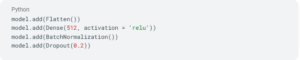
Upon defining the convolutional blocks, it is time to add a fully connected layer. To accomplish this, we’ll need to add two layers: Flatten and Dense. The Flatten layer reshapes the output of the last convolutional layer into a one-dimensional vector, preparing it for input to the fully connected layer, while the Dense layer, also known as the fully connected layer, is a layer where each neuron is connected to every neuron in the preceding layer, enabling the model to learn complex relationships between features extracted by convolutional layers. These 2 layers should be followed by another BatchNormalization and Dropout layers.

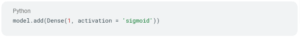
To conclude the structure of our model, we are just missing the output layer. This output layer will be another Dense layer with 1 unit and sigmoid as the activation function, since we are dealing with a binary classification (0 if it is a cat and 1 if it is a dog). If you had more animals that you wanted to classify, such as a cat, dog, bird, and fish, you would need to increase the units of your layer to 4 (the amount of different animal types) and change the activation function to softmax.

Now that the model structure has been defined, it is time to compile it. To do so, add a new cell with the following:

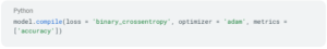
In this step, we define the loss function which is a crucial component that quantifies the difference between the predicted outputs of the model and the actual target values, the optimizer which is in charge of updating the parameters of a neural network during the training process to minimize the loss function, and the metrics which are functions that are used to evaluate the performance of your model. In a scenario where you were dealing with more than 2 types of animals, you should use categorical_crossentropy instead of binary_crossentropy.

We are almost ready to train our model, but first let’s define some callback functions that will be called during the training process to improve it:

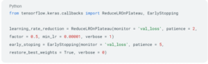
The first callback (ReduceLROnPlateau) will reduce the learning rate when the metric that is being monitored (val_loss) stops improving, according to the factor, until it reaches the minimum allowed value (min_lr). The learning rate determines how far the neural network weights change within the context of optimization while minimizing the loss function.
The second callback (EarlyStopping) stops the training process and restores the best weights when the metric that is being monitored (val_loss) stops improving.

Now we can start the training of our model by doing:

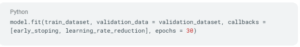
In the code above, we pass the training set, validation set, callbacks, and number of epochs. Each epoch represents a complete pass through the whole training dataset. In our scenario, we specified that we will loop through the training dataset 30 times unless the EarlyStopping callback is called. Keep in mind that for the callbacks we defined, the patience parameter denotes the number of epochs, meaning that if the metric being tracked does not improve after 5 consecutive epochs, the EarlyStopping callback will be invoked.

Congratulations, you have now trained your model and it is time to test it out and do some predictions with it.

Predictions

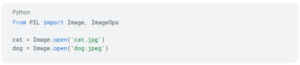
Before we use our model, let’s first download two images, one from a cat and another from a dog and save them. In case you are using Google Collab you can upload them by pressing the following button: 

Now let’s load our images and process them to a format suitable for our model. To load the images, do the following:

Once you have your images loaded, let’s convert them to grayscale and resize them to 128 pixels of width and 128 pixels of height.

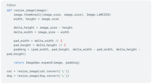
The conversion to grayscale is via the convert(‘L’) function, while the resizing of the image is taken care of using the resize_image function. Similar to what image_dataset_from_directory does, the resize_function pads the image to avoid deformation.

Now, the only missing steps are to reshape the images and run the model on them. To reshape images, run the following code:

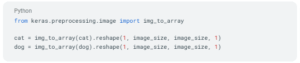
Your images are now ready to be used by the model. To do so add two new cells, one for each image.

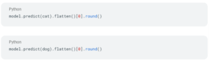
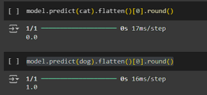
And here we have it: we ran our model with the two images. Hopefully, it gave you a value of 0 for the cat image and a value of 1 for the dog image. If not, the model might need some extra training 😅

Conclusion

As seen, the AI landscape is vast and full of intricacies and concepts. Hopefully, this article not only helped you understand better how AI evolved and how it works but also inspired you to dive deeper into it. Remember, even though this article is quite extensive, we have only scratched the surface, and there is so much more to learn and explore.